On the second day of 100 days of AI, we're diving into one of the fundamental optimization algorithms used in machine learning: Gradient Descent. Gradient Descent is a first-order iterative optimization algorithm used to find the minimum of a function. In the context of machine learning, this function is often a cost function that represents the difference between the predicted and actual values in a model.

What is Gradient Descent ?

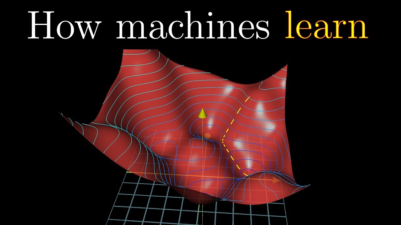
Imagine you're blindfolded on a weird, lumpy landscape, trying to find the lowest point without falling over. You can only sense if you're going downhill or uphill. Gradient Descent is like this quirky adventure, but for finding the lowest point of a wacky mathematical "hill" that represents how wrong our guesses are. Instead of feeling the terrain, we use math to figure out which way is downhill, and then we take tiny, careful steps in that direction until we hit the bottom. It's like teaching a computer to dance its way to the best answers in a game or recognize cats in pictures — it's all about finding that sweet spot where things just work!

Okay! That's not a technical definition of it. For people who love more technical definitions, Gradient Descent is an iterative optimization algorithm used to minimize a function by moving in the direction of the steepest descent, as defined by the negative of the gradient. The gradient represents the slope of the function at a given point, and moving in the opposite direction of the gradient allows us to descend toward the minimum of the function.

In machine learning, this function is often a cost function that measures the difference between predicted and actual values. By iteratively adjusting the parameters of a model in the direction that decreases the cost function the most, Gradient Descent effectively optimizes the model's performance.

There are different variants of Gradient Descent, such as Batch Gradient Descent, Stochastic Gradient Descent, and Mini-batch Gradient Descent (we will discuss about each of them in next series of posts), each with its own trade-offs in terms of computational efficiency and convergence speed. Overall, Gradient Descent is a fundamental tool for training machine learning models and is widely used in various optimization problems across different domains.

Enough of definitions. It's time to work on it.

Requirements of Gradient Descent

Gradient Descent doesn't work for all functions. It has it's own requirements that needs to be satisfied by the function. They are:

1. Differentiability
2. Convexity (for global minimum)

Differentiability

What does it mean ? Well, The function to be minimized must be differentiable, meaning its derivative exists at every point where it's being optimized -- not all functions meet these criteria.

Let's see some example functions that meet this criteria.

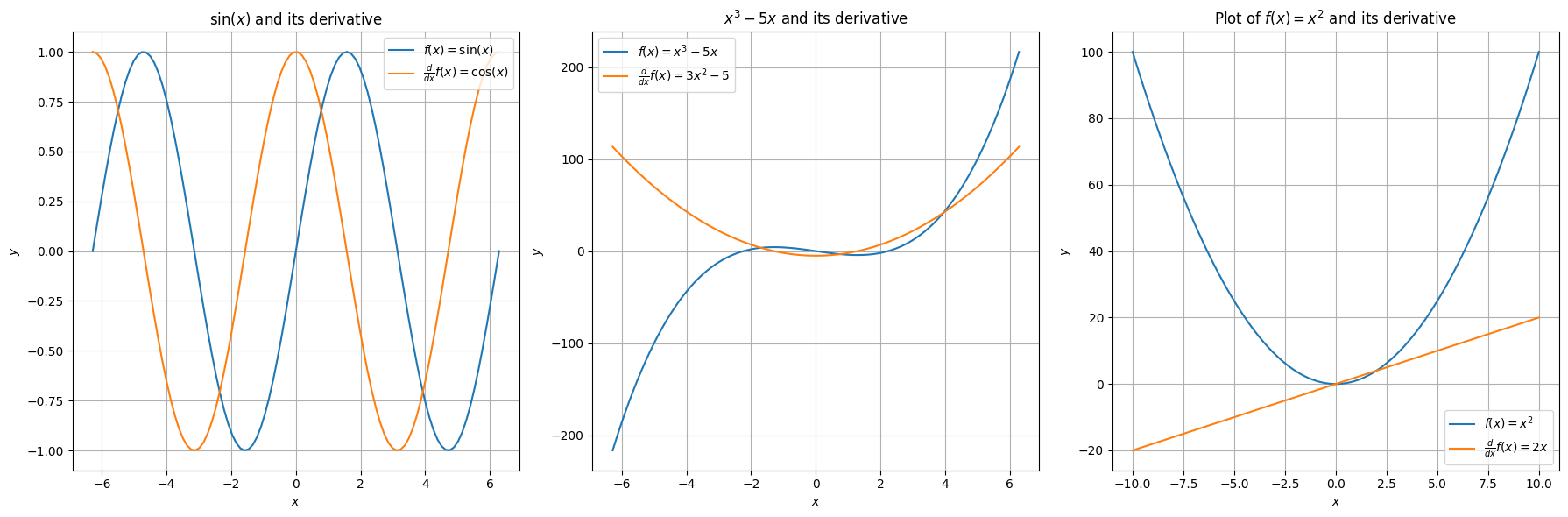
Where as, non-differentiable functions have a step a cusp or a discontinuity:

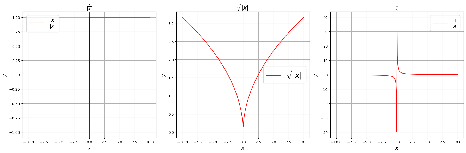
by now, you might have an idea about Differentiability of a function. The next requirement is Convexity.

Convexity

If the goal is to find the global minimum, the function should be convex, meaning it has a single minimum that Gradient Descent can converge to.

• A function $$f(x)$$ is said to be convex over an interval if, for any two points $$x1$$ and $$x2$$ in that interval, the line segment connecting the points lies above the graph of the function:

where $$0 \leq \lambda \leq 1$$ This property is known as Jensen's inequality.

• Geometrically, a function is convex if its graph does not curve downward. In other words, if you draw a line between any two points on the graph, the line lies above the graph itself.
• Another way to check mathematically if a univariate function is convex is to calculate the second derivative and check if its value is always bigger than 0.

Let's move on.

But what is a Gradient ?

In the context of Gradient Descent, the "gradient" is a vector that contains the partial derivatives of a function with respect to each of its variables. For example, if you have a function $$f(x, y)$$, its gradient $$\nabla f$$ is a vector $$\left( \frac{\partial f}{\partial x}, \frac{\partial f}{\partial y} \right)$$. This vector points in the direction of the steepest increase of the function at a specific point.

When you're using Gradient Descent to minimize a function $$f(W)$$, where $$W$$ is a vector of parameters (like weights in a machine learning model), you want to find the values of $$W$$ that minimize $$f$$. To do this, you start with an initial guess for $$W$$ and then update it iteratively using the gradient.

The update rule is:

Here, $$\alpha$$ is the learning rate, which controls how big the steps are that we take in the direction of the negative gradient. By subtracting, $$\alpha \nabla f(W_{old})$$ from $$W^{old}$$ we're effectively moving in the direction opposite to the gradient, which is the direction of the steepest decrease of the function.

By repeating this process, updating $$W$$ with each step, you gradually descend towards the minimum of the function. The gradient provides the direction for each step, helping you navigate towards the lowest point (minimum) of the function.

Significance of Learning Rate

The learning rate ($$\alpha$$) is a crucial hyperparameter in the Gradient Descent algorithm that determines the size of the steps taken during each iteration towards minimizing the loss function. Here's the significance of the learning rate:

• Controls Step Size: The learning rate dictates how much the parameters (weights) of the model should be adjusted with each iteration. A larger learning rate means taking larger steps, while a smaller learning rate means taking smaller steps.

• Impact on Convergence: The choice of learning rate can significantly impact the convergence of the algorithm. If the learning rate is too large, the algorithm may overshoot the minimum and fail to converge. On the other hand, if the learning rate is too small, the algorithm may take too long to converge or get stuck in a local minimum.

• Trade-off between Speed and Accuracy: A higher learning rate can lead to faster convergence, but it may also cause oscillations or overshooting around the minimum. Conversely, a lower learning rate may converge more slowly but with greater stability.

• Sensitive to Scale: The learning rate is sensitive to the scale of the input features and the magnitude of the gradients. Rescaling the features or using techniques like batch normalization can help in choosing an appropriate learning rate.

• Hyperparameter Tuning: Selecting an optimal learning rate often involves hyperparameter tuning. It is common to experiment with different learning rates to find the one that results in the fastest convergence without oscillations or divergence.

• Adaptive Learning Rates: There are variations of Gradient Descent, such as AdaGrad, RMSprop, and Adam, which adapt the learning rate during training based on the history of gradients. These adaptive methods can often converge faster and more reliably than using a fixed learning rate.

at this point, you have a solid understanding of Gradient Descent. Let's get our hands dirty by implementing it from scratch in Python.

Python Implementation

let's take a simple quadratic function, $$f(x) = x^2 + 5x + 6$$ and optimise it.

function to optimise:

derivative of the function:

let's code it.

import numpy as np
import matplotlib.pyplot as plt

def gradient_descent(function_to_optimize,
                     derivative,
                     lr: float = 0.1,
                     initial_x: float = -6.5,  # random
                     iterations: int = 50):
    x_values = [initial_x]
    costs = [function_to_optimize(initial_x)]
    
    for i in range(iterations):
        current_x = x_values[-1]
        gradient = derivative(current_x)
        new_x = current_x - lr * gradient
        
        x_values.append(new_x)
        costs.append(function_to_optimize(new_x))
        
    return x_values, costs, lr, iterations

let's create anotehr function that helps us to animate the Gradient Descent Optimisation

import matplotlib.animation as animation

def create_animation(x_values, costs, lr, iterations, function_to_optimize):
    fig, ax = plt.subplots(figsize=(10, 6))
    plt.grid()
    ax.set_xlim(-7, 2)
    ax.set_ylim(-1, 20)
    ax.set_xlabel('x')
    ax.set_ylabel('y')
    ax.set_title(f'Gradient Descent Optimization, lr = {lr}')

    # init empty plots for function and optimization process
    x = np.linspace(-7, 2, 100)
    y = function_to_optimize(x)
    function_line, = ax.plot(x, y, 'r-', label='Function to Optimize')
    optimization_line, = ax.plot([], [], 'bo-', label='Gradient Descent Optimization')

    # Update function for animation
    def update(frame):
        optimization_line.set_data(x_values[:frame+1], costs[:frame+1])
        return optimization_line,

    ani = animation.FuncAnimation(fig, update, frames=iterations, blit=True)
    plt.legend(handles=[function_line, optimization_line], loc='upper right')
    ani.save(f'gradient_descent_animation_{lr}.gif', writer='pillow', fps=5)
    plt.show()

let's play with these functions

Plots at different learning rates

def function_to_optimize(x):
    return x**2 + 5*x + 6

def derivative(x):
    return 2*x + 5

x_values, costs, lr, iterations = gradient_descent(function_to_optimize, derivative)

create_animation(x_values, costs, lr, iterations, function_to_optimize)

learning rate = 0.1

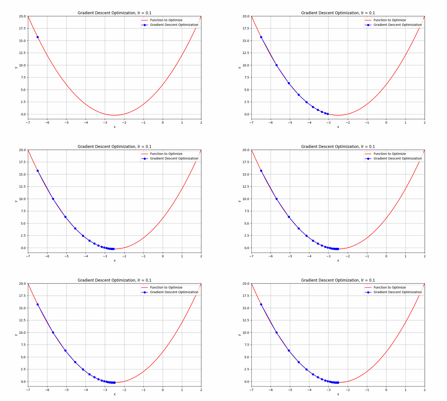
just play with the learning rate parameter in the gradient_descent function and see how learning rate affects the optimisation. also you can play with different functions and iterations and see how it goes.

as you can see, when learning rate set to 0.1, the optimisation tries to reach the minimum point and takes more steps to reach there. let's try with slightly higher learning rate 0.3.

learning rate = 0.3

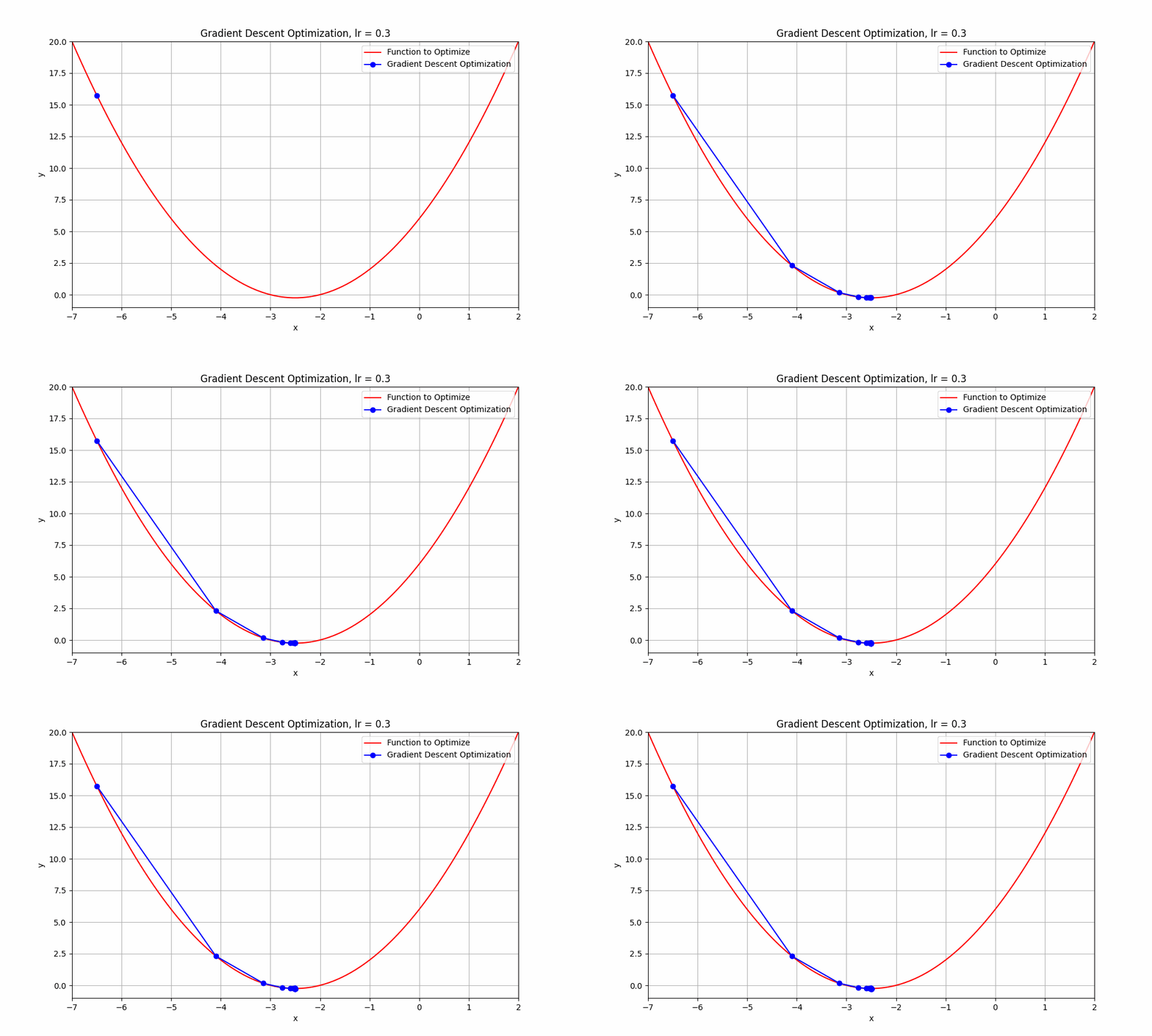
it starts from the initial point and takes a huge jump downward to reach the minimum. you can say this obvisouly took less steps.

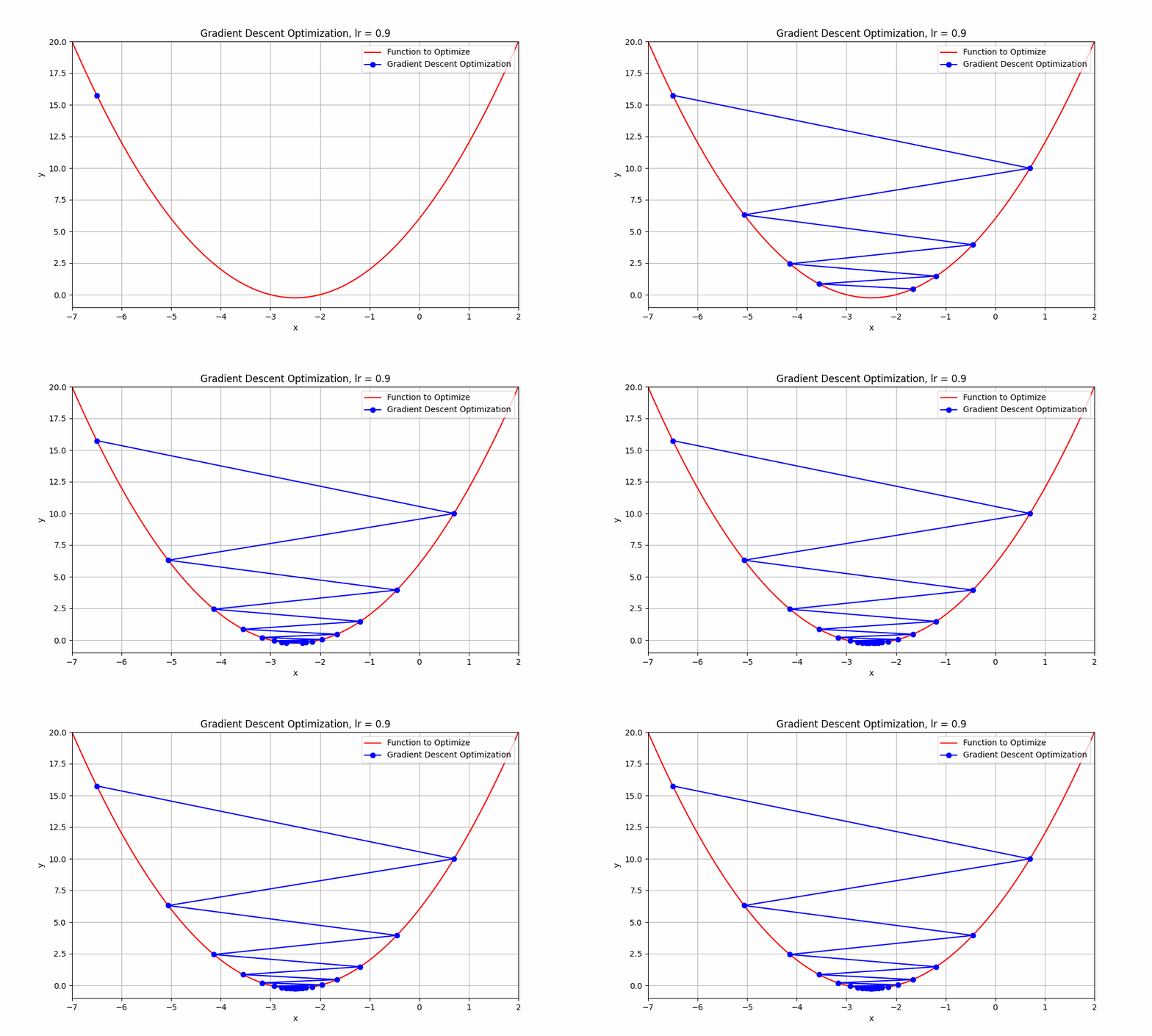
let's have a look at an interesting case, learning rate = 0.9

learning rate = 0.9

What just happend there?

Well, it means that we're taking relatively large steps towards the minimum of our loss function. The negative and positive steps we're observing indicate that the algorithm is overshooting the minimum and then oscillating around it.

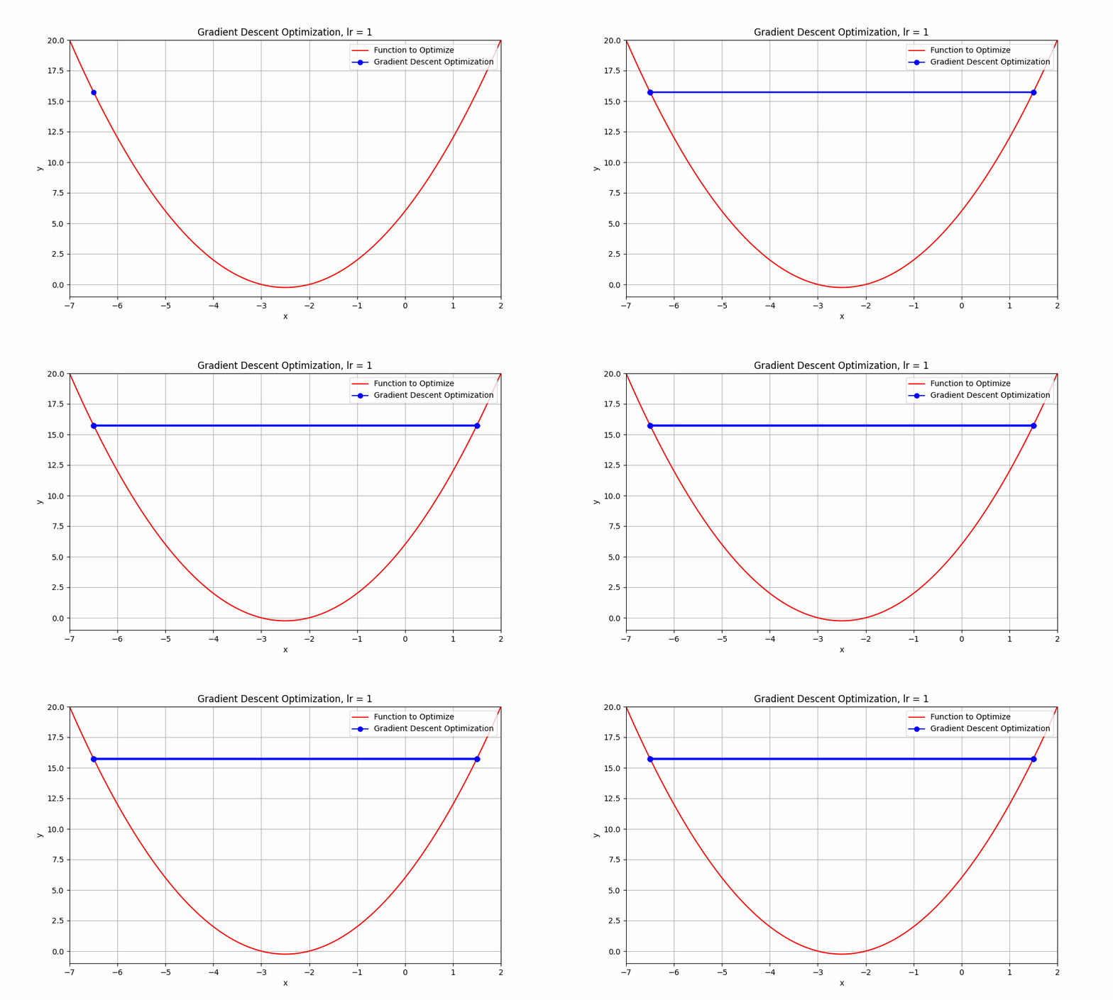
what happends if we go beyond 0.9 ? let's set learning rate = 1.0

learning rate = 1.0

This doesn't even reach the minumum point. it just oscialtes between negative and positive.

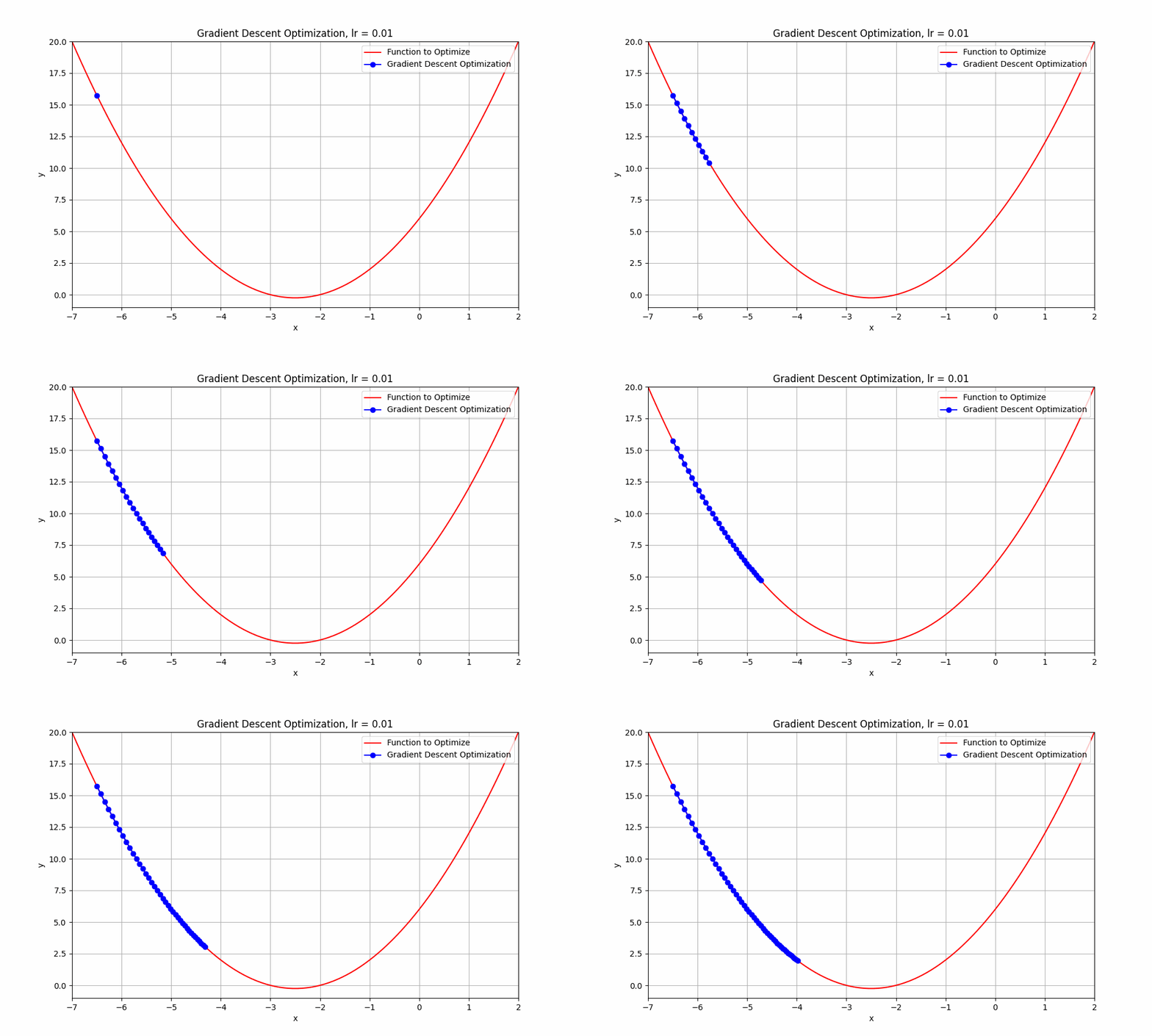
let's set our learning rate very low, something like 0.01, what do you think happens to our algorithm ? Let's have a look.

learning rate = 0.01

well this too, did not reach its destination. it stopped midway. But hey, you might think that it's going downhill but why did it stop? well, it ran out of fuel. just kidding, it stopped because iterations are not enough to reach the minimum. if we do this for more iterations, it will reach eventually.

So, to conclude, it's always recommended to keep the learing rate at optimum value. Not too low, or not too high. it's not something that is fixed for different set of problems. you just have to play with that and see what works best. That's why we have several other Optimising methods in Gradient Descent that optimises the learning rate. We will learn about them in next upcomming series. Stay tuned and that's all for now. G'Day.

In upcomming posts, we will see more hands on Gradio demos to let you guys play with the models right here.